Forward and Inverse Kinematics | 09.06.2018
Forward and inverse kinematics were the most important software systems of my Smart Lamp project.
Control of the lamp arm has two layers; the lowest level control layer that manages the PWM interface with the servos, and the kinematics layer, which is responsible for calculating how the arm needs to move to bring the light, or end-effector, to a desired position.
The kinematics layer has two parts, forward and inverse. Forward kinematics (FK), calculates the position of the end-effector given the position of each of link in the arm. Inverse kinematics (IK), does the opposite, it solves for the position of the arm given a goal position of the end-effector.
The kinematics system I wrote for this project is based on the Denavit-Hartenberg convention. Denavit-Hartenberg is a method for describing the positions of links in an arm, and is commonly used in robot kinematics.
Under the Denavit-Hartenberg convention each link is assigned a frame of reference according to a set of rules:
- The Zi-1axis must be the axis of actuation for joint i.
- The Xi axis must be perpendicular to and intersect the Zi-1 axis.
- The Yi axis is derived from Zi and Xi per the right-hand-rule.
In the case of Smart Lamp’s arm they look like this:
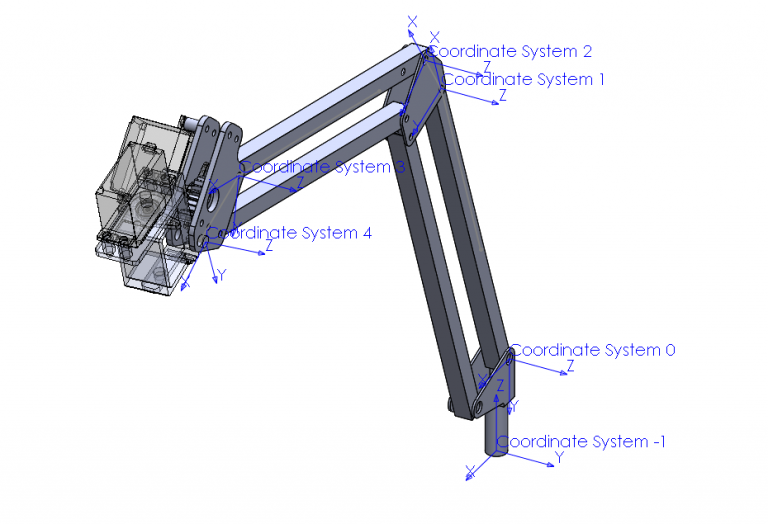
Once these frames are established each link’s position can be defined relative to the previous link using four parameters:
a– Link Length – Distance from joint (i-1) to (i) on the Xi axis
α– Link Twist – Angle between Zi-1 axis and Zi axis about the Xi axis
d– Link Offset – Distance from joint (i-1) to (i) on the Zi-1 axis
θ– Joint Angle – Angle between Xi-1 axis and Xi axis about the Zi-1 axis
Parameters d (Link Offset) and θ (Joint Angle) are the “joint variables” for a link and respectively represent prismatic and revolute actuation.
To solve the forward kinematics problem, these parameters are plugged into a homogeneous transformation matrix for each link. The homogeneous transform matrix is the product of four transformation matrices, rotation about Z(i-1), translation along Z(i-1), rotation about Xi, and translation along Xi.
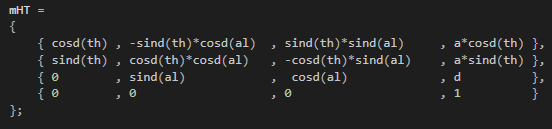
By multiplying the homogeneous transform matrices together the position of the end effector can be found with respect to the frame of reference associated with any previous link in the kinematic chain.
The last part of my FK system is handling the parallelogram four-bar joints in our arm. This type linkage causes the next link in the chain to rotate as the previous link moves, such that its angle relative to the floor remains fixed. The animations below demonstrate how this behavior differs between a regular joint and a four-bar linkage:
To account for this in the FK system, the two four-bar links are flagged and whenever their position is updated they rotate the subsequent link an equal and opposite amount, to match the behavior of the real mechanism.
Solving IK is more complicated. For FK there is only one solution for any configuration of the arm; However for IK there can be multiple, one or no solutions for any desired position of the end-effector. I decided to use a rudimentary method called gradient following, which was acceptable for the scope of this project.
In this example, the arm needs to move from it’s current position at (13.7, 12.4) to a goal position of (8.0, 8.0).
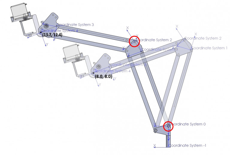
To solve this problem the gradient following method tests how manipulating each joint affects distance from the goal position. The contour plot below shows the configuration space of the arm in this example. The axes represent the position of joints 1 & 3 (circled in red above), and the colors show distance in inches from the goal position at that point.
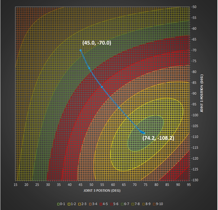
By incrementing each joint independently and simulating the new position using the FK system the software can measure how adjusting each axis affects distance to the target. Using these measurements the software finds a new point closer to the goal, and repeats the process, while scaling down the increment as it approaches the goal.
Looking at the blue line on the plot you can see how it “follows the gradient” of the configuration space to find the solution.